Why circular statistics matter - the case of respiratory signals

import numpy as np
import matplotlib.pyplot as plt
from matplotlib.collections import LineCollection
from matplotlib.colors import Normalize
import matplotlib.cm as cm

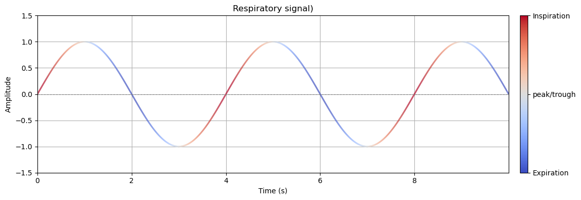
Respiration is inherently rhythmic, consisting of two distinct phases: inspiration and expiration.

Respiration can be measured using different devices, but is often measured with a belt sensitive to pressure placed around the abdomen. As such the signal measured is higher when the abdomen is expanded, compared to contracted. Interpreting such a through traditional linear methods can obscure important temporal and physiological distinctions.

Consider a simple sinusoidal signal used to represent the respiratory cycle as measured using a respiration belt. At two time points with identical amplitude values, one may occur during inspiration and the other during expiration. From a purely linear standpoint, these points are indistinguishable. However, from a biological perspective, they represent fundamentally different physiological states: differential brainstem activity, sensory gating, or cortical excitability, for example, are often phase-locked to either inspiration or expiration.

To demonstrate this, let’s first generate a sinusoidal signal representing a few respiratory cycles!

# Settings
fs = 1000  # Sampling frequency in Hz
duration = 15  # seconds
t = np.linspace(0, duration, fs * duration, endpoint=False)
freq = 0.25  # respiration-like frequency in Hz (4s cycle)
resp_signal = np.sin(2 * np.pi * freq * t)

Then we plot

# compute slope (derivative) for colormap
dresp = np.gradient(resp_signal)

# normalise for color mapping
slope_max = np.max(np.abs(dresp))
norm = Normalize(vmin=-slope_max, vmax=slope_max)
colors = cm.coolwarm(norm(dresp))

# prepare line segments
points = np.array([t, resp_signal]).T.reshape(-1, 1, 2)
segments = np.concatenate([points[:-1], points[1:]], axis=1)
lc = LineCollection(segments, colors=colors[:-1], linewidths=2)

# Plot
fig, ax = plt.subplots(figsize=(12, 4))
ax.add_collection(lc)
ax.set_xlim(t.min(), t.max())
ax.set_ylim(-1.5, 1.5)
ax.axhline(0, color='gray', linestyle='--', linewidth=0.8)
ax.set_title("Respiratory signal)")
ax.set_xlabel("Time (s)")
ax.set_ylabel("Amplitude")
ax.grid(True)

# Colorbar with custom ticks and labels
sm = cm.ScalarMappable(norm=norm, cmap='coolwarm')
sm.set_array([])
cbar = plt.colorbar(sm, ax=ax, orientation='vertical', pad=0.02)

# Custom tick positions and labels
tick_locs = [-slope_max, 0, slope_max]
tick_labels = ['Expiration', 'peak/trough', 'Inspiration']
cbar.set_ticks(tick_locs)
cbar.set_ticklabels(tick_labels)


plt.tight_layout()
plt.show()

import numpy as np
import matplotlib.pyplot as plt
from matplotlib.collections import LineCollection
from matplotlib.colors import Normalize
import matplotlib.cm as cm

# Settings
fs = 1000  # Sampling frequency in Hz
duration = 10  # seconds
t = np.linspace(0, duration, fs * duration, endpoint=False)
freq = 0.25  # respiration-like frequency in Hz (4s cycle)
resp_signal = np.sin(2 * np.pi * freq * t)
dresp = np.gradient(resp_signal)

# Normalize slope for color mapping
slope_max = np.max(np.abs(dresp))
norm = Normalize(vmin=-slope_max, vmax=slope_max)
colors = cm.coolwarm(norm(dresp))

# Build colored segments
points = np.array([t, resp_signal]).T.reshape(-1, 1, 2)
segments = np.concatenate([points[:-1], points[1:]], axis=1)
lc = LineCollection(segments, colors=colors[:-1], linewidths=2)

# Plot setup
fig, ax = plt.subplots(figsize=(12, 4))
ax.add_collection(lc)
ax.set_xlim(t.min(), t.max())
ax.set_ylim(-1.5, 1.5)
ax.axhline(0, color='gray', linestyle='--', linewidth=0.8)
ax.set_title("Respiratory signal", fontsize=14, pad=10)
ax.set_xlabel("Time (s)", fontsize=12)
ax.set_ylabel("Amplitude", fontsize=12)

# Minimal styling
ax.grid(False)
ax.spines['top'].set_visible(False)
ax.spines['right'].set_visible(False)
ax.spines['left'].set_linewidth(0.8)
ax.spines['bottom'].set_linewidth(0.8)
ax.tick_params(width=0.8)

# Helper to calculate slope angle using wider window
def compute_slope_angle(t_target, t, y, window_ms=100):
    window_samples = int((window_ms / 1000) * fs)
    idx = np.argmin(np.abs(t - t_target))
    idx1 = max(idx - window_samples, 0)
    idx2 = min(idx + window_samples, len(t) - 1)
    dx = t[idx2] - t[idx1]
    dy = y[idx2] - y[idx1]
    angle = np.degrees(np.arctan2(dy, dx))
    return angle, t[idx], y[idx]

# Expiration label at x = 2
angle_exp, x_exp, y_exp = compute_slope_angle(2, t, resp_signal)
ax.text(x_exp, y_exp, "Expiration", fontsize=11, rotation=angle_exp,
        color='blue', va='top', ha='center', fontweight='medium')

# Inspiration label at x = 4
angle_insp, x_insp, y_insp = compute_slope_angle(4, t, resp_signal)
ax.text(x_insp, y_insp, "Inspiration", fontsize=11, rotation=angle_insp,
        color='red', va='bottom', ha='center', fontweight='medium')

plt.tight_layout()
plt.show()

Caveats of the hilbert transform used in this notebook

• link to other notebook